The Core Question
Most AI systems ask:
Can we predict what will go viral?
Prediction assumes trends are passive - something we observe after they emerge.
But trends are not passive.
They are shaped by decisions:
- who sees content first
- when it is posted
- how it is amplified
- where visibility expands
So the real question becomes:
Can we optimize the conditions under which trends emerge?
This is where Bayesian Optimization (BO) enters.
The Big Idea
Instead of treating virality as a prediction problem, we treat it as a black-box optimization problem.
Traditional pipeline:
Data → Model → Prediction
New pipeline:
Decision → Propagation → Feedback → Optimization → Better Decision
The shift is subtle - but profound.
We move from observing trends to engineering them.
Trends as Propagation Systems
A trend doesn’t appear instantly. It propagates through stages.
1. Engagement Initiation
Early signals emerge:
- likes
- comments
- shares
- watch time
These become a feature vector:
‘x ∈ ℝ^d’
2. Amplification
Influencers and network structure drive spread:
- resharing velocity
- high-degree nodes
- algorithmic boosts
Amplification introduces uncertainty - exactly what BO exploits.
3. Visibility Expansion
Algorithms increase exposure:
- explore pages
- trending feeds
- recommendations
This stage determines whether content dies or explodes.
4. Virality
Sustained exponential spread occurs across the network.
This becomes the optimization target.
The Optimization Problem
Instead of predicting virality directly:
‘max_{x ∈ X} f(x)’
Where:
- x = trend seeding strategy
- f(x) = influence spread (unknown)
We cannot write this function analytically.
We can only evaluate it.
That makes it a perfect black-box optimization problem.
Influence Spread as the Objective
We evaluate f(x) using the Independent Cascade (IC) model.
Independent Cascade Simulation
- Seed nodes activate.
- Activated nodes attempt to activate neighbors with probability (p_{uv}).
- Process repeats until no new activations occur.
Expected influence:
‘f(x) = E_IC[Reach(S_x)]’
Estimated using Monte Carlo simulations.
Each evaluation is expensive - which is exactly where BO shines.
Bayesian Optimization Core
Surrogate Model
‘f(x) ~ GP(μ(x), k(x, x’))’
Gaussian Processes model:
- predicted influence
- uncertainty over unknown regions
Acquisition Function
‘a(x) = μ(x) + κ σ(x)’
This balances:
- exploitation (high-performing strategies)
- exploration (uncertain but promising strategies)
Sequential Loop
- Evaluate initial strategies
- Train GP surrogate
- Optimize acquisition function
- Test new strategy
- Update model
- Repeat
Optimization becomes intelligent exploration.
Visualizing the Process
IC Spread Simulation
flowchart LR
  %% Time-layered IC spread (t0 -> t1 -> t2 -> t3)

  subgraph T0["t0 - seeds"]
    direction TB
    S1((S1)):::seed
    S2((S2)):::seed
  end

  subgraph T1["t1 - newly activated"]
    direction TB
    A1((A1)):::active
    A2((A2)):::active
    A3((A3)):::active
  end

  subgraph T2["t2 - newly activated"]
    direction TB
    B1((B1)):::active
    B2((B2)):::active
    B3((B3)):::active
    B4((B4)):::active
  end

  subgraph T3["t3 - newly activated"]
    direction TB
    C1((C1)):::active
    C2((C2)):::active
  end

  %% Propagation edges with probabilities (example p_uv)
  S1 -- "p=0.35" --> A1
  S1 -- "p=0.22" --> A2
  S2 -- "p=0.40" --> A2
  S2 -- "p=0.18" --> A3

  A1 -- "p=0.30" --> B1
  A1 -- "p=0.12" --> B2
  A2 -- "p=0.28" --> B2
  A2 -- "p=0.20" --> B3
  A3 -- "p=0.25" --> B4

  B2 -- "p=0.15" --> C1
  B3 -- "p=0.33" --> C1
  B4 -- "p=0.19" --> C2

  %% Styling
  classDef seed fill:#ff6b6b,stroke:#111,color:#fff,stroke-width:1px;
  classDef active fill:#4dabf7,stroke:#111,color:#fff,stroke-width:1px;
Acquisition Function Evolution
How BO decisions evolve over iterations:
- uncertainty decreases
- exploration shifts toward promising regions
Search Space Trajectory
flowchart TB
  %% "Heatmap-style" BO convergence (Mermaid can't render true heatmaps,
  %% so we approximate with a colored grid + a trajectory overlay)

  subgraph H["Search Space Heatmap (approx) - BO converges toward higher values"]
    direction TB

    %% Row 1 (low to medium)
    subgraph R1[" "]
      direction LR
      A11[" "]:::v1
      A12[" "]:::v2
      A13[" "]:::v2
      A14[" "]:::v3
      A15[" "]:::v3
    end

    %% Row 2
    subgraph R2[" "]
      direction LR
      A21[" "]:::v2
      A22[" "]:::v2
      A23[" "]:::v3
      A24[" "]:::v4
      A25[" "]:::v4
    end

    %% Row 3
    subgraph R3[" "]
      direction LR
      A31[" "]:::v2
      A32[" "]:::v3
      A33[" "]:::v4
      A34[" "]:::v5
      A35[" "]:::v6
    end

    %% Row 4
    subgraph R4[" "]
      direction LR
      A41[" "]:::v3
      A42[" "]:::v4
      A43[" "]:::v5
      A44[" "]:::v6
      A45[" "]:::v7
    end

    %% Row 5 (high region / optimum neighborhood)
    subgraph R5[" "]
      direction LR
      A51[" "]:::v3
      A52[" "]:::v5
      A53[" "]:::v6
      A54[" "]:::v7
      A55[" "]:::v8
    end
  end

  %% BO evaluation trajectory overlay (sample points over iterations)
  A11 -->|t1| A22 -->|t2| A33 -->|t3| A44 -->|t4| A55

  %% Color scale (cool -> hot)
  classDef v1 fill:#e8f4ff,stroke:#9dbfe6,stroke-width:1px;
  classDef v2 fill:#cfe8ff,stroke:#9dbfe6,stroke-width:1px;
  classDef v3 fill:#a8d2ff,stroke:#7aaee6,stroke-width:1px;
  classDef v4 fill:#7ab6ff,stroke:#5a95de,stroke-width:1px;
  classDef v5 fill:#4b97ff,stroke:#2f6fce,stroke-width:1px,color:#fff;
  classDef v6 fill:#2d7be6,stroke:#1f5fb8,stroke-width:1px,color:#fff;
  classDef v7 fill:#1f5fb8,stroke:#164787,stroke-width:1px,color:#fff;
  classDef v8 fill:#163a66,stroke:#0f2745,stroke-width:1px,color:#fff;
Performance vs. Random Seeding (Why BO Wins)
A simple baseline for trend seeding is random selection:
- pick seed users randomly (or randomly choose strategy knobs like time/hashtags/influencer tier)
- run the propagation simulation (IC / Monte Carlo)
- record reach / engagement / virality
This is appealing because it is easy and unbiased - but it is extremely inefficient in large combinatorial spaces.
Bayesian Optimization (BO) improves over random by learning from every evaluation and deciding where to test next using a surrogate model + acquisition function. In high-noise propagation problems, this often yields stronger performance under a fixed evaluation budget.
What we compare
Assume the objective is expected reach:
‘f(x) = E_IC[Reach(S_x)]’
We compare two methods under the same budget (N):
- Random: sample (x1, x2,….., xN) uniformly from the strategy space
- BO: adaptively choose (x_{t+1} = \arg\max a(x)) after each evaluation
Metrics used for comparison
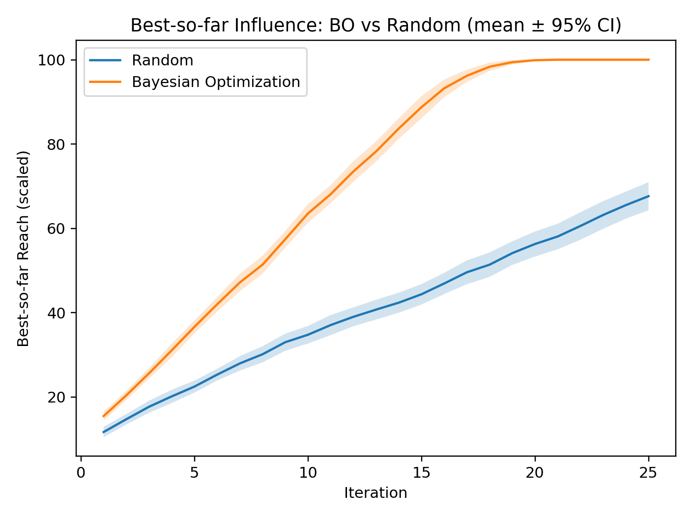
- Best-So-Far Influence (Simple & Strong)
Measures progress as optimization proceeds:
‘BestSoFar(t) = max_{i ≤ t} f(x_i)’
BO should rise faster and reach higher values with fewer evaluations.
- Area Under the Best-So-Far Curve (AUBC)
A single-number summary of sample efficiency:
‘AUBC = Σ_{t=1}^{N} BestSoFar(t)’
Higher AUBC means you achieved strong performance earlier and consistently.
- Regret (Optimization Lens)
If we assume the true optimum is (f(x^*)), the simple regret is:
‘r_N = f(x*) − max_{t ≤ N} f(x_t)’
BO should yield lower regret under equal budgets.
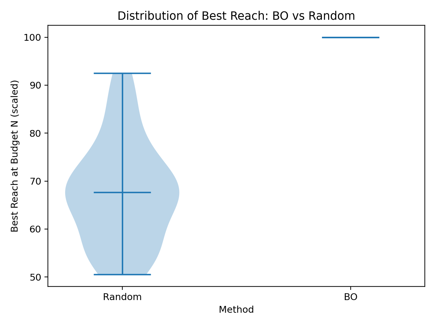
- Stability Under Noise (Propagation Variance)
Since MCST is stochastic, compare variance:
‘Var(f(x)) ≈ (1 / (K − 1)) Σ_{k=1}^{K} ( Reach_k(S_x) − Ȓeach(S_x) )²’
BO can incorporate uncertainty and avoid being misled by noisy single samples.
1) Convergence: Best-So-Far Reach vs Iterations
This diagram shows the typical qualitative behavior: BO climbs faster than random.
graph LR

subgraph Iterations
I1["Iter 1"] --> I2["Iter 2"] --> I3["Iter 3"] --> I4["Iter 4"] --> I5["Iter 5"]
end

subgraph Random
R1["10"] --> R2["18"] --> R3["22"] --> R4["28"] --> R5["31"]
end

subgraph BO
B1["10"] --> B2["25"] --> B3["40"] --> B4["55"] --> B5["65"]
end

I1 --- R1
I2 --- R2
I3 --- R3
I4 --- R4
I5 --- R5

I1 --- B1
I2 --- B2
I3 --- B3
I4 --- B4
I5 --- B5
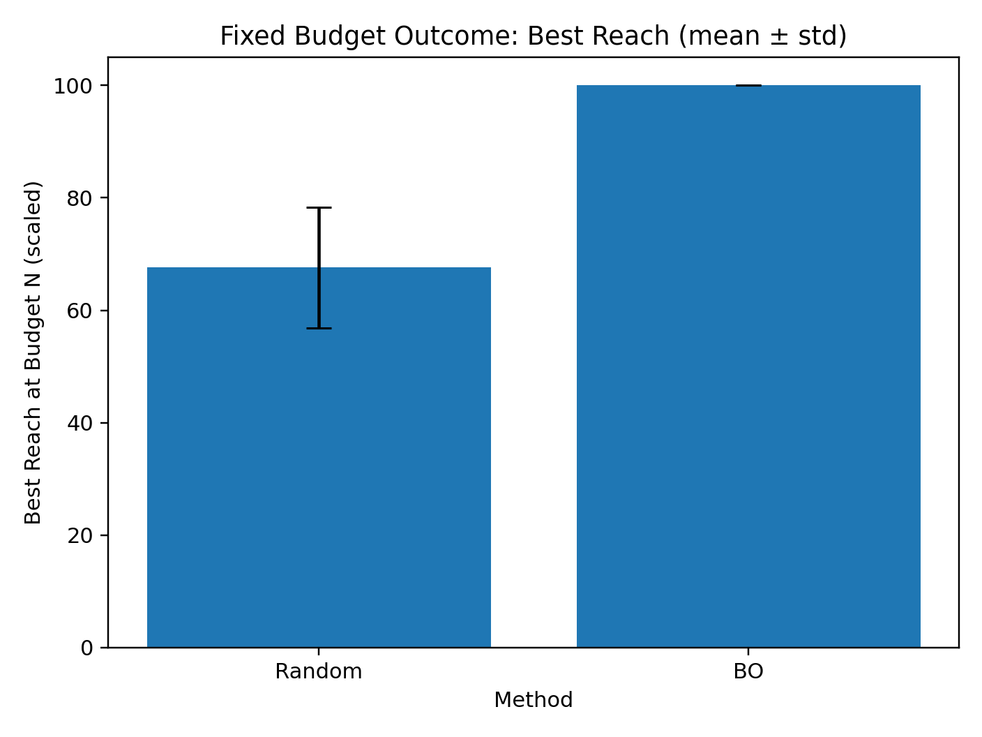
2) Budget Efficiency: Same Budget, Different Outcome
With a fixed evaluation budget (e.g., 20 simulations), BO typically discovers a higher-performing strategy.
flowchart LR
  R["Random\nBest Reach ≈ 55"]:::low --> C["Fixed Budget (N evals)"]
  B["BO\nBest Reach ≈ 85"]:::high --> C

  classDef low fill:#ffd6d6,stroke:#111,color:#111;
  classDef high fill:#d6f5d6,stroke:#111,color:#111;
3) Why Random Fails: Search Space Explosion
Random sampling wastes many evaluations in low-performing regions.
flowchart LR
    A["Huge Strategy Space X"] --> B["Random picks mostly low/medium zones"]
    A --> C["BO builds surrogate f̂(x) + uncertainty"]
    C --> D["Acquisition picks high-potential regions"]
    D --> E["Faster discovery of strong seeding strategies"]
Under the same evaluation budget (N), • BO should achieve higher BestSoFar reach • higher AUBC • lower simple regret • and often more stable improvement under Monte Carlo noise.
A realistic target framing for synthetic IC experiments: • BO improves best reach by ~20–50% vs random under tight budgets (e.g., 20–50 evaluations), depending on: • network structure • seed set size • noise level (number of MC rollouts per evaluation) • dimensionality of strategy space
Performance vs Random Seeding (Figures)
Best-so-far convergence (mean ± 95% CI)
Fixed-budget outcome (bar chart)
Distribution of best reach (violin plot)
Real-Graph Research Artifact: Higgs Retweet Network
The synthetic IC figures above explain the optimization intuition. The research-artifact version uses the SNAP Higgs retweet graph: 223,833 nodes, 308,596 edges, and a seed budget of k = 20.
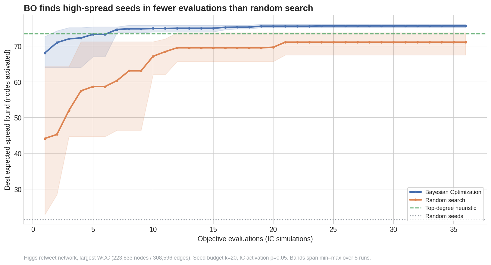
Real data: BO reaches the high-spread region in fewer evaluations than random search, while top-degree remains an extremely strong baseline.
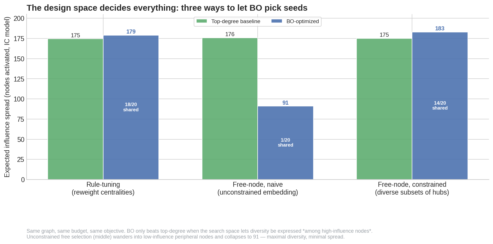
The actual lesson is structural: the search-space design decides whether BO refines a strong heuristic, collapses, or finds a better diverse subset.
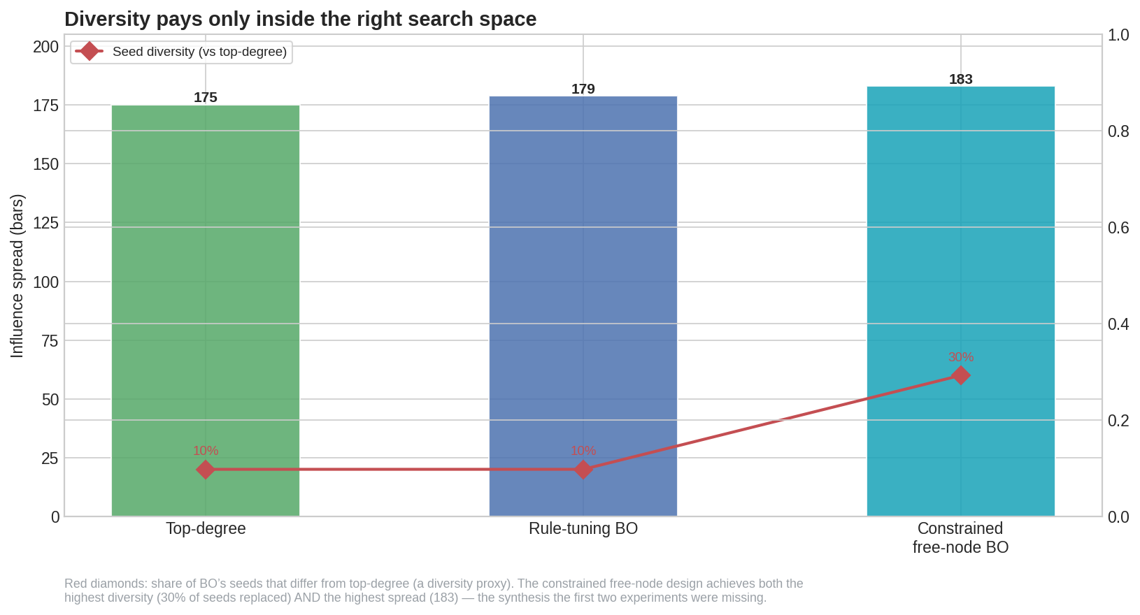
Diversity only pays when it is constrained to nodes that can actually carry a cascade.
For the full build log and limitations, see Influence Maximization using BO.
Approach B: The Same Network, Different People
There is a methodological weakness in the experiment above.
The Higgs topology is real. The behavior moving through it is not.
Independent Cascade models commonly give every eligible edge the same activation probability, or draw those probabilities from an arbitrary distribution. That is useful for isolating graph structure. It also assumes that everybody is equally likely to activate on every kind of content.
They are not.
A technically literate node should not respond to an ML paper in the same way it responds to a sports clip. A highly social, video-oriented node may reverse that ordering. So Approach B replaces the single global probability with a topic-conditional one:
| ‘logit p(u → v | c) = logit p₀ + β₁ affinity(v,c) + β₂ share(v) + β₃ similarity(u,v,c)’ |
The persona signals come from the public MatrAIx release, which exposes 1,290 categorical dimensions spanning technical familiarity, interests, psychology, lifestyle, and media behavior. The first implementation builds two deliberately different content profiles:
- an ML paper, using machine-learning familiarity, technology and science interest, technical literacy, need for cognition, and reading preference;
- a sports clip, using sports interest, sports exposure, video preference, excitement seeking, and social-media attitude.
BO now searches over four interpretable weights: topology, topic affinity, sharing propensity, and neighborhood redundancy. The question becomes more specific:
Which structurally strong nodes are plausible first adopters for this particular content?
The conditioning problem is part of the model
There is no identity join between a MatrAIx persona and an anonymous Higgs node. Randomly sampling 223,833 global personas would not recreate Twitter’s user distribution during the July 2012 Higgs discovery. Pretending otherwise would turn synthetic enrichment into fake ground truth.
So the implementation treats persona assignment as an explicit sensitivity parameter. It runs three assumptions about how strongly a node’s observed graph activity aligns with a sampled persona’s platform-fit score:
0.00: random assignment;0.35: weak alignment;0.70: strong-alignment stress test.
A result that disappears across this grid is assumption-sensitive, not robust.
The initial audit of the 999-row decoded public sample found 665 age-eligible records and an effective sample size of 652.8 after soft conditioning. The requested fields are usable but incomplete: coverage ranges from 18.0% to 77.0%. The ML-paper and sports-clip affinity scores are meaningfully distinct in the sample (correlation = -0.225). That is enough to run the mechanism as a synthetic sensitivity experiment. It is not evidence about the actual preferences of Higgs users.
Three-tier provenance
| Layer | What it is | What can be claimed |
|---|---|---|
| Network | Real SNAP Higgs retweet topology | The edges and graph structure are observed data |
| People and behavior | Synthetic persona-to-node assignments and assumed activation coefficients | A controlled modeling scenario, not reconstructed user behavior |
| Method | Heterogeneous IC simulation, Monte Carlo evaluation, and Gaussian-process BO | A reproducible topic-conditional influence-maximization method |
Even a human-grounded MatrAIx record becomes synthetic metadata once it is assigned to an anonymous graph node. The honest output is therefore a robustness study over assumptions, not a claim that the model discovered who those Twitter users really were.
The implementation, conditioning audit, tests, and reporting contract are in the Approach B research artifact. The full 223,833-node performance result is intentionally not reported until the cached Higgs graph is supplied and every conditioning value is run.
Why This Is Innovative
Bayesian Optimization is commonly used for:
- protein synthesis
- material discovery
- hyperparameter tuning
This work applies BO to:
Social influence optimization
Key innovation:
- trends become optimization landscapes
- virality becomes an objective function
- strategy becomes a decision variable
Why Not Reinforcement Learning?
RL works best when:
- dense rewards exist
- continuous interaction is available
Here:
- evaluations are expensive
- rewards are delayed
- sample efficiency matters
BO provides better uncertainty-aware exploration.
RL becomes a future extension.
Challenges & Limitations
No idea is perfect.
Key challenges include:
- high evaluation noise from Monte Carlo simulations
- local traps in optimization space
- high-dimensional strategy vectors
- GP scalability limitations
These motivate future research directions.
Notes / Caveats • BO can be misled by noise if (K) is too small (not enough MC rollouts). • BO may fall into local traps if exploration is too low. • Random can look competitive in extremely high noise or poorly specified search spaces.
So comparisons will include: • confidence intervals over multiple runs (repeat experiments with different random seeds) • optionally varying (K) (MC rollouts) to show robustness.
The Deeper Insight
Traditional view
BO optimizes vectors.
New view
BO navigates complex social decision spaces.
This reframes social systems as:
- structured optimization landscapes
- sequential experimentation environments
The Mathematical Engine Behind Trend Optimization
At the heart of this system is a precise mathematical framework that turns social propagation into an optimization problem. Below is a conceptual breakdown of each core equation and how it connects to virality engineering.
1. Estimating Influence Spread
‘E_IC[Reach(S_x)] ≈ (1 / K) Σ_{k=1}^{K} Reach_k(S_x)’
This equation approximates the expected influence spread under the Independent Cascade (IC) model.
- (S_x) = seed set selected by strategy (x)
- {Reach}_k(S_x)) = number of activated nodes in simulation (k)
- (K) = number of Monte Carlo simulations
Because influence propagation is stochastic, we simulate it multiple times and average the results. This gives us a stable estimate of expected virality.
Each evaluation is computationally expensive - making Bayesian Optimization ideal.
2. Constructing the Virality Score
‘ViralityScore(x) = Σ_i w_i · f_i(x)’
Virality is not a single signal - it is a weighted combination of measurable engagement features:
- (f_i(x)) = engagement feature (e.g., share velocity, clustering coefficient, watch-time retention)
- (w_i) = learned importance weight
This linear aggregation transforms raw social signals into a structured objective function.
3. Learning Optimal Feature Weights
‘L(w) = - Σ_{t=1}^{T} ( y_t - Σ_i w_i f_i(x_t) )²’
This loss function learns weights (w_i) that best align predicted virality with observed viral outcomes.
- (y_t) = observed virality outcome at time (t)
- (x_t) = strategy used
- (T) = number of training instances
The negative squared error formulation allows us to optimize weights using Bayesian Optimization itself, refining how virality is computed.
4. Acquisition Functions (Decision Rule)
Bayesian Optimization does not optimize the true function directly. It optimizes a surrogate model and uses acquisition functions to choose the next evaluation.
Expected Improvement (EI)
‘a_EI(x) = E[ max(0, f(x) - f(x⁺)) ]’
- f(x⁺) = best observed value so far
EI chooses strategies expected to outperform the current best - balancing exploration and exploitation.
Upper Confidence Bound (UCB)
‘a_UCB(x) = μ(x) + κ σ(x)’
- μ(x) = predicted mean
- σ(x) = uncertainty
- κ = exploration parameter
UCB explicitly trades off:
- Exploitation (high predicted influence)
- Exploration (high uncertainty)
5. Strategy Selection
‘x* = argmax_{x ∈ X} a(x)’
The next strategy tested is the one that maximizes the acquisition function.
This is the core decision-making step in Bayesian Optimization.
6. Gaussian Process Kernel Functions
The surrogate model uses kernels to measure similarity between strategies.
Radial Basis Function (RBF)
| ‘k_RBF(x, x’) = exp( - | x - x’ | ² / (2ℓ²) )’ |
- Smooth, infinitely differentiable
- Assumes gradual changes in influence landscape
- Controlled by length-scale (\ell)
Matérn Kernel
| ‘k_Matern(x, x’) = (2^(1-ν) / Γ(ν)) · ( (√(2ν) | x - x’ | ) / ℓ )^ν · K_ν( (√(2ν) | x - x’ | ) / ℓ )’ |
- More flexible than RBF
- Better suited for noisy, less smooth social systems
- Controlled by smoothness parameter (\nu)
7. Edge Activation Probability
‘p_uv’
This represents the probability that an activated node (u) activates neighbor (v) in the Independent Cascade model.
These probabilities encode:
- strength of connection
- historical interaction frequency
- platform-specific influence likelihood
Why This Matters
These equations collectively transform:
- engagement signals
- network structure
- uncertainty
- propagation randomness
into a sequential optimization framework.
Rather than predicting trends passively, this framework:
- Models uncertainty over virality
- Selects promising strategies
- Learns from outcomes
- Improves future decisions
The mathematics is not just descriptive - it is prescriptive.
It enables AI to navigate social systems intelligently.
Future Directions
Where this research can go next:
- Graph Neural Network surrogates
- RL-based adaptive strategies
- Multi-fidelity Bayesian Optimization
- Dynamic, evolving social graphs
- Real-time autonomous trend engineering
This is where sequential decision-making and BO begin to merge.
The Big Idea - Final Thought
Most systems try to predict trends after they happen.
This work asks something different:
What if AI could learn how to create them?
By combining influence propagation models with Bayesian Optimization, we move from passive forecasting toward active, uncertainty-aware decision making.
Sometimes optimization isn’t about finding the answer.
It’s about learning how to move through the space.
References
- Kempe et al. (2003). Maximizing the Spread of Influence through a Social Network
- Snoek et al. (2012). Practical Bayesian Optimization
- García-Hernández et al. (2022). Bayesian Optimization for Influence Maximization
- Liang (2024). Bayesian Optimization of Functions over Node Subsets in Graphs
Author Note
Written as part of my exploration in AI for Sequential Decision Making
MS Data Science - University of Minnesota
After the last line
Comments & sharing
Agree, disagree, add context, or send this to someone who would have a take.
Share
Public thread
Comments are public and attached to this post through GitHub Discussions. Sign in with GitHub to join the thread.
Open public discussions